⚙️ Process Scheduling & Process States
4. Process Scheduling Introduction
🎯 Why Process Scheduling? To maximize CPU utilization by switching between processes
when current process waits for I/O or time expires.
Process Scheduling Overview
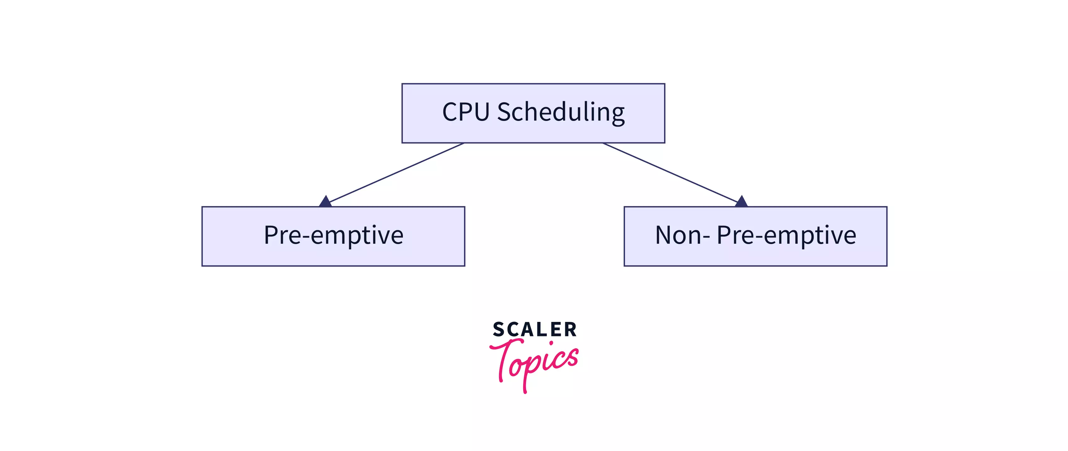
| Scheduling Type | Preemptive | Non-Preemptive |
|---|---|---|
| CPU Control | OS can forcibly take CPU | Process voluntarily gives up CPU |
| Starvation | Less starvation | More starvation possible |
| CPU Utilization | High | Low |
| Examples | Round Robin, Priority | FCFS, SJF |
Important Formulas:
Turnaround Time (TAT) = Completion Time - Arrival Time
Waiting Time (WT) = Turnaround Time - Burst Time
Response Time = First CPU allocation time - Arrival Time
Turnaround Time (TAT) = Completion Time - Arrival Time
Waiting Time (WT) = Turnaround Time - Burst Time
Response Time = First CPU allocation time - Arrival Time
🎯 3. Goals of CPU Scheduling
- Maximize CPU Utilization: Keep the CPU as busy as possible.
- Maximize Throughput: Complete as many processes as possible in a given time.
- Minimize Waiting Time: Reduce the time a process spends in the ready queue.
- Minimize Turnaround Time: Complete each process as fast as possible (from submission to completion).
- Minimize Response Time: Quickly start responding to interactive processes (like keyboard input).
- Fairness: Ensure no process is starved or left waiting too long.
📌 Note: CPU scheduling is crucial for multitasking and responsiveness in an
operating system. Different algorithms (like FCFS, SJF, Round Robin) try to achieve these goals
differently.
5. FCFS (First Come First Serve)
🎯 Interview Point: FCFS is simplest scheduling algorithm - processes are executed in
order of arrival. Main problem is Convoy Effect.
Example: Processes P1(24), P2(3), P3(3) - numbers are burst times
FCFS Gantt Chart
P1
P1
P1
P1
P2
P3
0242730
| Process | Arrival Time | Burst Time | Completion Time | TAT | WT |
|---|---|---|---|---|---|
| P1 | 0 | 24 | 24 | 24 | 0 |
| P2 | 0 | 3 | 27 | 27 | 24 |
| P3 | 0 | 3 | 30 | 30 | 27 |
Average WT = (0 + 24 + 27) / 3 = 17
Convoy Effect: Short processes wait behind long processes, like fast cars stuck behind
slow truck on single-lane road.
🌍 Real World: Bank queue - first customer takes long time, others wait regardless of
their quick transactions.
6. SJF (Shortest Job First)
🎯 Interview Key Point: SJF gives minimum average waiting time. Problem is predicting
burst time and starvation of long processes.
Same Example: P1(24), P2(3), P3(3) - but scheduled by burst time
SJF Gantt Chart
P2
P3
P1
P1
P1
P1
03630
| Process | Burst Time | Completion Time | TAT | WT |
|---|---|---|---|---|
| P2 | 3 | 3 | 3 | 0 |
| P3 | 3 | 6 | 6 | 3 |
| P1 | 24 | 30 | 30 | 6 |
Average WT = (0 + 3 + 6) / 3 = 3
SJF Problems:
- Starvation: Long processes may never execute
- Prediction: Impossible to know exact burst time
- Convoy Effect: If first process is long (non-preemptive)
🌍 Real World: Hospital emergency room - quick checkups done before major surgeries.
7. Priority Scheduling
🎯 Interview Point: Each process has priority. Higher priority executes first. SJF is
special case where priority = 1/burst_time.
Example: P1(10,3), P2(1,1), P3(2,4), P4(1,5) - (burst_time, priority)
Priority Scheduling Gantt Chart
P2
P3
P3
P1
P1
P4
0131314
Starvation Problem: Low priority processes may never execute.
Solution - Aging: Gradually increase priority of waiting processes.
Solution - Aging: Gradually increase priority of waiting processes.
Aging Implementation:
Every 15 minutes:
for each process in ready queue:
if (waiting_time > 15 minutes):
priority = priority + 1
🌍 Real World: Airport boarding - first class boards first, but if economy passengers
wait too long, they get priority (aging).
8. Round Robin (RR)
🎯 Interview Favorite: Most popular scheduling algorithm. FCFS + preemption with time
quantum. No starvation, fair to all processes.
Example: P1(24), P2(3), P3(3) with Time Quantum = 4
Round Robin Gantt Chart (TQ = 4)
P1
P1
P2
P3
P1
P1
P1
P1
047101418222630
| Process | Burst Time | Completion Time | TAT | WT |
|---|---|---|---|---|
| P1 | 24 | 30 | 30 | 6 |
| P2 | 3 | 7 | 7 | 4 |
| P3 | 3 | 10 | 10 | 7 |
Average WT = (6 + 4 + 7) / 3 = 5.67
Time Quantum Selection:
- Too Small: High context switching overhead
- Too Large: Becomes FCFS
- Optimal: 80% processes complete within one time quantum
🌍 Real World: Time-sharing computer systems - each user gets CPU for fixed time, then
switches to next user.
9. Multi-Level Queue (MLQ)
🎯 Interview Point: Ready queue divided into multiple queues based on process type.
Each queue has its own scheduling algorithm.
Multi-Level Queue Structure
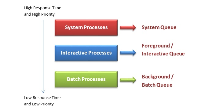
System Processes:
P1
P2
Highest Priority - FCFS
Interactive:
P3
P4
P5
Medium Priority - RR
Batch Processes:
P6
P7
Lowest Priority - FCFS
MLQ Problems:
- Starvation: Lower priority queues may never execute
- Inflexibility: Process can't move between queues
- Convoy Effect: Present in lower priority queues
🌍 Real World: Office hierarchy - CEO tasks get immediate attention, manager tasks
next, employee tasks last.
10. Multi-Level Feedback Queue (MLFQ)
🎯
Interview Point: MLFQ allows processes to move between queues based on behavior. More
flexible than MLQ.
Multi-Level Feedback Queue Structure
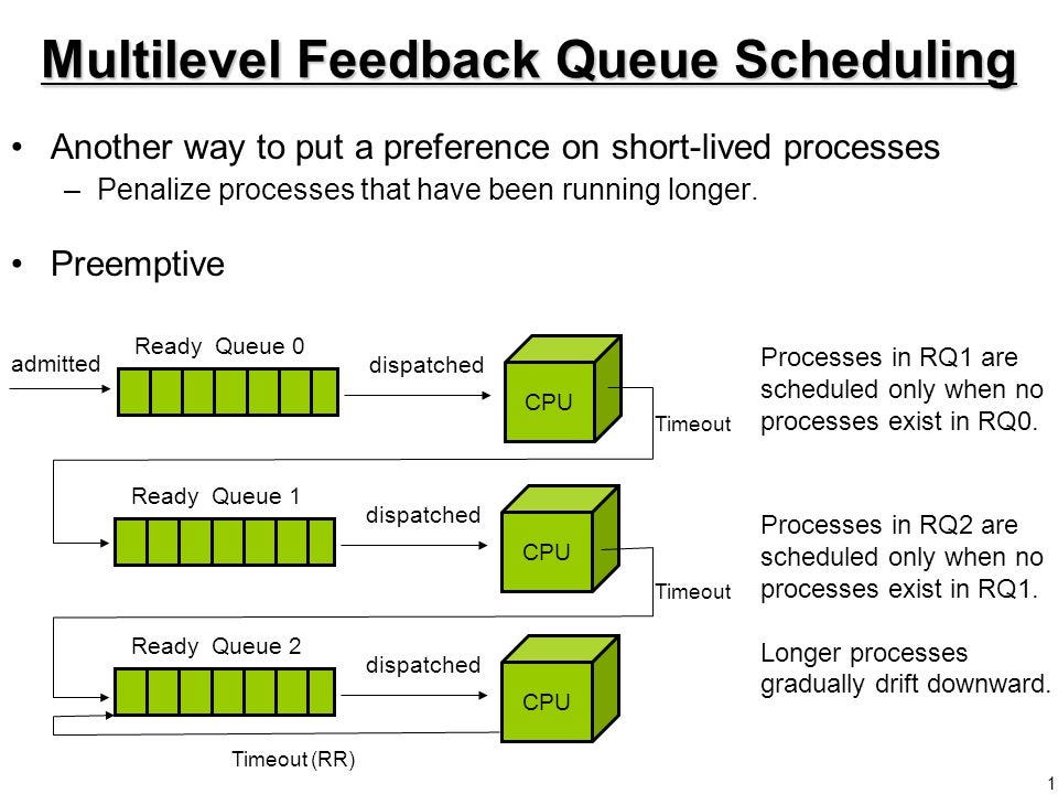
High Priority Queue:
P1
P2
Time Quantum = 4
Medium Priority Queue:
P3
P4
Time Quantum = 8
Low Priority Queue:
P5
P6
Time Quantum = 16
MLFQ Problems:
- Complexity: Difficult to implement and tune
- Starvation: Low priority processes may still starve
- Convoy Effect: Can occur in lower priority queues
🌍 Real World: University grading system - students can retake exams (move up) or fail
and take remedial classes (move down).
Conclusion
Process scheduling is a critical aspect of operating systems, ensuring efficient CPU utilization and responsiveness. Understanding various scheduling algorithms helps in designing better systems.